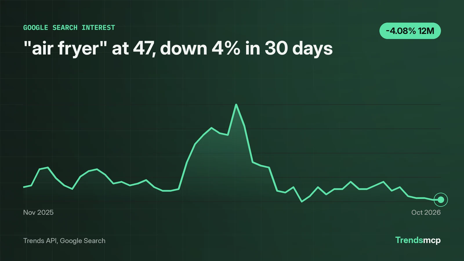
A trend graph plots search interest on a 0-100 index, where 100 marks the highest week in the displayed window, not a count of searches. Read any trend graph in three passes. First, the level: where the latest point sits against the peak. Second, the slope: percent change over fixed windows, because eyes misjudge curves. Third, the shape: repeating humps are seasonality, and lone spikes need outside evidence. The worked example here is live Google Search data for "air fryer": 47 for the week of October 31 2026, down 4% in 30 days and down 4% year over year, with November humps near 65 every year since 2022 and a 100 print in May 2026 that the graph alone cannot explain. Data pulled November 3 2026.
100 is the peak of the window, not a headcount
On the "air fryer" graph, 100 labels the week of May 9 2026, the highest week in the 261-week window. Every other point is a percentage of that week. The latest reading of 47 means roughly 47% of the peak week's search volume, not 47 searches, not 47 thousand. There are no absolute counts on this graph at all.
Change the window and the same week gets a different number. A 1-year graph renormalizes 100 to the highest week inside that year; a 5-year graph renormalizes to the highest week in five years. This is why screenshots of trend graphs without visible dates mislead: the shape survives, the scale does not.
One more trap. Each separately pulled series normalizes to its own peak. The query "search trends" also printed 100 in the week of May 9 2026, but that is each series' own maximum, not a shared scale. The two 100s are not comparable quantities. Never overlay two separately normalized series and read the gap between them as a real gap.
Your eyes will misread the slope, so quote a fixed window
"air fryer" fell from 49 to 47 in the 30 days to October 31 2026, a 4.08% decline that looks almost flat on the graph. It is still a real number, computed point to point by get_growth, and it is the number to quote. The 90-day window reads minus 11.32%, from 53 on August 1 to 47. The 12-month window reads minus 4.08%, from 49 on November 1 2025 to 47.
Eyeballing the curve between August and October suggests a steeper fall than 11% supports, because the eye weighs the jagged weekly moves more than the endpoints. The fix is a habit: always quote the window, both endpoint values with their dates, and the percent. "Down 4% in 30 days (49 on October 3 to 47 on October 31)" can be checked. "Sloping down lately" cannot. One caveat on the method: get_growth computes point to point, endpoint week against endpoint week, not an average of the window. A single odd week at either end can swing the percent, which is why quoting both endpoint values matters as much as quoting the percent.
Small moves on flat-looking graphs still matter. A 4% monthly drift compounded over a year is a different story than a flat line, and only the fixed window shows which one you are looking at. The last four weeks read 48, 48, 47, 47: genuinely flat heading into the holiday ramp, which makes the coming November print a clean test of whether the seasonal pattern still holds.
A repeating hump is seasonality; a lone spike is just a spike
Late November prints for "air fryer" read 65, 67, 65, and 65 across 2022 through 2025, each in the week of Thanksgiving. A second, smaller hump follows around December 27 to 31: 70, 68, 62, and 60 in those years. That is seasonality with a shape, not just a direction: two humps, one for buying and one for unboxing-season cooking, repeating four years running. A graph earns the right to a seasonal claim only when the hump repeats, and this one does. Expect the next one, and do not write a news story about it.
The May 9 2026 print of 100 is the opposite case. It has no repeat anywhere in the 261-week record, and the series contains no cause for it. The rule from the newsroom applies to graphs too: say what moved, then cite why, and when you cannot cite why, say that plainly. A spike is not proof that an event happened. It is proof that searches spiked, and the next step is reporting, not assumption.
Also mind the cadence. Keyword history on this source is weekly; the latest point always covers a full week ending October 31 2026, not this morning. Live boards are different: they carry an as_of_ts timestamp, like November 3 2026 09:01 UTC on the current Google Trends board. Neither is a tick. Do not ask a weekly series for hourly moves.
The two calls that drew this graph
In Claude with Trends MCP, ask with "using TrendsMCP" so the model routes to the tools instead of a web search:
get_time_series(keyword="air fryer", source="google search")
get_growth(keyword="air fryer", source="google search", percent_growth=["30D", "90D", "12M"])
Over REST, one key works for both:
POST https://api.trendsmcp.ai/api
{"mode": "get_time_series", "keyword": "air fryer", "source": "google search"}
The time series endpoint returns the weekly points behind the chart. The growth endpoint computes the point-to-point windows, so no slope gets eyeballed. A probe of the nonsense keyword "xqzwjklmno qqq" returned zeros across all 261 weekly points, growth of 0.0 marked flat, and a data_quality flag of low warning that the signal is over 90% zero values. Read the flag, not just the line: zeros mean "no data," not "no interest." Source notes live on the Google Search data page, and the Python tutorial shows the same pulls in code. Underlying search data belongs to Google; see Google Trends.